ArcGIS Velocity IoT Integration: Manhole and Sewer Telemetry Into a Feature Layer
At 03:10 on a wet February morning, a water-level alarm from manhole MH-2291 reached Priya Raman’s phone two hours before the pump station upstream began to surcharge. Priya runs the GIS for Pinewood, a water utility with 4,200 manhole covers. Eight hundred of them report telemetry, and that single alarm changed how her city funds underground infrastructure.
The uncomfortable part is that the hard part wasn’t the map or the alarm rule. For an ArcGIS Velocity IoT integration, it was the 300 bytes her device sends from a concrete pit every fifteen minutes, and whether those bytes survive the trip into a layer her analysts can query.
Most ArcGIS Velocity advice starts inside the Velocity interface. That’s the easy hop. This guide starts underground instead, then walks the whole path: what the device should transmit, how the feed is configured, how the analytic is built, and the two configuration traps that break deployments quietly.
Wiring sensors into a GIS layer and need hardware you can specify with confidence? See the Black Ant smart manhole cover range that publishes this telemetry natively.
What ArcGIS Velocity IoT Integration Actually Does

ArcGIS Velocity is Esri’s real-time and big data analytics capability for IoT data. It ingests, processes, visualises, stores, and acts on streaming observations, then publishes the results as map layers, dashboards, alerts, or writes to external systems.
It runs in two deployment shapes, plus one honest alternative. ArcGIS Online SaaS is fully managed and includes both real-time and big data analytics. Velocity for ArcGIS Enterprise, self-hosted from Enterprise 12.1 onward, is real-time only and excludes big data analytics, which Esri scoped to match what GeoEvent Server did. The third option is a non-Esri stack: QGIS, PostGIS, and GeoServer consume the same MQTT stream, and roughly 50 lines of middleware replaces the managed service.
That third option isn’t a footnote. Plenty of municipal programmes can’t justify an ArcGIS Online subscription plus a Velocity licence for a few hundred stationary sensors. This article assumes you’ve picked streaming and want the implementation. If you haven’t made that call yet, the GIS integration for smart manhole monitoring guide compares REST push, MQTT middleware, and batch import side by side.
The Four Components of a Real-Time Analytic
Every real-time analytic is built from the same four pieces. Get this model straight and the rest of the tool becomes navigable.
| Component | What it is | Examples in Velocity | What it means for a sensor fleet |
|---|---|---|---|
| Feed | A live inbound stream from an external source | MQTT, Kafka, HTTP, RabbitMQ, Azure IoT Hub, AWS IoT, Cisco IoT | One feed per broker connection, not per device |
| Data source | Secondary data loaded for enrichment, never the live stream | A hosted feature layer of manholes, a boundary polygon layer | The asset register you join against |
| Tool | Processing and analysis steps chained together | Map Fields, Filter by Expression, Calculate Motion Statistics, Detect Incidents, Join Features | Separates signal from noise and detects events |
| Output | The destination for each processed event | Feature Layer (new), Feature Layer (existing), Stream Layer, email, HTTP, Teams, Kafka | Where the analyst actually sees the result |
The most common misunderstanding is the second row. A data source is not your live telemetry. It’s the static or slowly-changing dataset a tool joins to; sensor messages arrive through a feed, full stop.
Velocity tools also split into two families, and the split explains most configuration errors. Stateless tools judge each observation alone: filter a threshold, calculate a field. Stateful tools need history, operate on tracks rather than individual readings, and include Calculate Motion Statistics, Detect Incidents, Filter by Geometry, and Join Features.
Stateful tools use a Track Time Window to purge cached observations. Too short and level-trend detection sees nothing; too long and the analytic holds unneeded memory. For a manhole reporting every fifteen minutes, a 24-hour window captures a full fill-and-drain cycle.
What Your Field Device Must Send Before Anything Else

Every decision downstream of the sensor is constrained by choices made at the sensor: reporting interval, payload size, message rate, local buffering, and battery budget.
Message Rate, Battery Budget, and the Throughput Ceiling
Run the arithmetic before you talk to a salesperson. A fleet of 500 covers reporting every 15 minutes generates 48,000 messages a day, which averages 0.56 messages per second. Scale to 10,000 covers on the same cadence and you reach 960,000 messages a day, or about 11.1 messages per second.
Both numbers sit far below the event-rate ceiling on every Velocity tier. That tells you something the marketing pages don’t: payload size usually decides your licence tier, not device count. At 200-byte payloads, the Standard tier’s 25 KB/s ceiling supports roughly 128 events per second. At 1 KB payloads, the same tier supports roughly 25. Same licence, five times less headroom, purely from padding.
Battery budget pulls the opposite way. More frequent reporting means more radio time, and radio time dominates the power draw on a device that must run for years underground. A 15-minute cadence is a defensible compromise; a 30-second cadence needs a bigger cell, and the cell becomes the cost driver.
Insist on store-and-forward buffering too. A sensor that discards readings when the broker is unreachable makes Velocity look broken when it isn’t, and it destroys the historical record exactly when the event matters most. Ask suppliers to demonstrate buffering depth in messages and retention in hours, in writing.
Connecting the Feed: ArcGIS Velocity MQTT, Kafka, and the Cloud Platforms
Velocity offers more than 20 ready-to-use feed types in four categories. Knowing which category your device belongs to narrows the configuration to one screen.
| Feed category | Feed types | When it’s the right choice |
|---|---|---|
| ArcGIS | Feature layers, stream layers | Chaining Velocity onto an existing stream |
| Cloud | Azure IoT Hub, AWS IoT, Cisco IoT | Your organisation standardised on a cloud IoT platform |
| Web & Messaging | MQTT, Kafka, HTTP, RabbitMQ, RSS, Azure Event Hub | Most direct device integrations, including manhole fleets |
| Data Providers | Dataminr, Samsara, FlightAware, Baron Weather, CompassCom | Consuming a third party’s curated feed |
For a manhole deployment, Web and Messaging is almost always the answer, and MQTT is the specific choice. Six parameters decide whether the feed connects or fails silently.
- Host. Prefix with
ssl://for TLS ortcp://for plain TCP. Get this wrong and the connection appears to hang rather than error. - Port. Default is 8883 for TLS. Confirm your broker’s listening port rather than assuming.
- Username and password. Use a dedicated credential per feed, so you can revoke one integration without breaking the rest.
- Client ID. Must be unique per connected client. Two feeds sharing a Client ID disconnect each other in a loop, which looks like an unstable network.
- Topic. Where the messages stream. This is where most fleets get sloppy.
- QoS level. 0 is at most once, 1 is at least once, 2 is exactly once. QoS 1 is the usual compromise for environmental telemetry.
One flat topic such as iot kinect data works for a demo and collapses for a city. Put identity in the topic and measurements in the payload, then let the hierarchy carry the geography.
manhole/{region}/{district}/{device_id}/telemetry
manhole/{region}/{district}/{device_id}/alarm
A structure like this lets one analytic subscribe to a single district without filtering 40,000 messages in the pipeline, and it maps cleanly onto how municipalities already organise maintenance crews.
Building the Real-Time Analytic

With the payload clean and the feed connected, the analytic is mechanical. In the Analytics section, open the Real-Time Analytics page and create a new analytic from an existing feed.
- Attach the MQTT feed as the input.
- Add a data source for enrichment, typically your manhole feature layer or district boundaries.
- Connect Map Fields and align incoming fields to your target schema.
- Assign the TRACK ID tag to the device identity field.
- Add Filter by Expression for threshold conditions you want to discard early.
- Chain the stateful tool you need, such as Calculate Motion Statistics or Detect Incidents.
- Add the output, either Feature Layer (new), Feature Layer (existing), or Stream Layer.
- Name it, save it, and start it. A real-time analytic needs at least one input and one output before it can run.
Filter before you enrich, so you’re not joining records you’ll throw away.
Tools That Matter for Underground Telemetry
Four tools carry most of the work, and one is routinely misapplied.
Filter by Expression handles flat thresholds, such as tilt above 15 degrees or hydrogen sulphide above 10 ppm. Map Fields aligns your payload to the destination schema and applies the Track ID tag. Join Features enriches each reading with asset attributes, so an alarm arrives carrying the road class and structure depth. Calculate Motion Statistics is the tool everyone associates with vehicle speed, and the one nobody applies to a tank.
That omission is worth correcting. A water level changes slowly, so the interesting signal is the rate of change, not the instantaneous reading. Running motion statistics over a 24-hour track window turns a level into a fill rate in millimetres per hour, which is the number that tells an operator whether a basin is filling faster than the pumps can clear it. Same tool, different framing, and it converts a monitoring feed into a forecasting one.
The February 2026 Track ID Requirement
Here’s a change that breaks running analytics, and it’s almost undocumented in article form because it lives in a community announcement.
As of the February 2026 ArcGIS Velocity update, any real-time analytic that connects a feed to the join port of Join Features, Detect Incidents, Filter by Geometry, or Calculate Distance must include a Track ID field. Analytics that lack one are stopped and can’t be restarted until the error is fixed.
You have two remedies. Add a Track ID field to the join feed, or route that feed through Map Fields and tag an existing or new field as TRACK ID. Static data sources are unaffected, as are join feeds that already carry a Track ID.
Two properties belong on a wall. The Track ID must be unique, and null values degrade performance over time. On a manhole fleet, the correct Track ID is the stable device identity, not a timestamp and not a row number.
A Percentage-Change Alarm in Arcade
Velocity supports Arcade expressions for conditions, and those expressions can read up to 5 historical track observations. That’s enough to write a rise-rate alarm without external state.
var prev = $track.history[-1].level_mm;
var now  = $feature.level_mm;
if (prev == null) { return false; }
return (now - prev) / prev > 0.15;
Read that as “alert when the level has risen more than 15 percent since the previous observation.” Tune it per structure type. A deep trunk sewer and a shallow local connection don’t fill at the same rate, and one global threshold will either flood you with false alarms or miss the event that matters.
Geofencing and Alerting for Underground Assets
Geofencing compares target features against areas of interest, and the geofence features connect to the tool’s join port. That detail drives the configuration.
A static geofence is fixed geometry that doesn’t change while the analytic runs, such as a flood-prone basin polygon. Velocity offers a real performance advantage here: when geofences don’t change, a static data source is the best-performing option, because Velocity collects the join features once at start and doesn’t refresh them until the analytic restarts. For a manhole programme with stable geography, use static.
Dynamic geofencing
compares a target feed against an updating join feed, which suits areas of interest that move. Two constraints apply. The geofence dataset can’t exceed 768 MB, and the Join Time Window is required. Without an END TIME field, stale observations are purged from memory; with one, features age out per the END TIME value or the join window, whichever comes first.
The practical manhole pattern is concrete: dozens of drainage-basin polygons as a static source, Filter by Geometry or Detect Incidents joined against them, and one analytic per region so an alert storm in one district can’t starve the others.
Velocity routes alerts through more outputs than most teams use. Email covers the audit trail, and text messages via an externally accessible SMTP server reach the duty crew. HTTP outputs POST, PUT, or DELETE to external systems with Basic or OAuth 2.0 authentication, which is how a work-order system receives an alert without a human in the loop. Microsoft Teams and Slack accept webhook messages, and Amazon SNS handles fan-out to push, SMS, and email.
Choose deliberately. An operator who receives 40 alerts overnight stops reading them by week three. Route threshold breaches to the crew channel and reserve email for the daily digest.
Writing to the Feature Layer, and Two Traps Nobody Mentions

| Output | What it does | Use it when |
|---|---|---|
| Feature Layer (new) | Creates the target layer from the incoming schema | Piloting, or the data has no home yet |
| Feature Layer (existing) | Writes into a layer you already own | The manhole layer is also the asset layer, the usual case |
| Stream Layer | Publishes live state, optionally keeping the latest observation per Track ID | You need current condition on a map, not a history table |
The Feature Layer (existing) output has schema rules that trip people up. The incoming data and the destination must generally match on geometry type and spatial reference, and every incoming field must exist in the destination. The destination may have extra fields, and that’s how enrichment persists.
Use Map Fields to align the two. The TRACK ID and START TIME tags don’t have to match those in the destination when you’re writing to ArcGIS Online or ArcGIS Server feature layers.
One option is quietly important. You choose between add all new features and keep only the latest feature for each Track ID value. The second behaves like update-in-place and is the correct setting for an asset register, where MH-2291 should be one row that gets refreshed rather than 96 rows a day.
The Stream Layer output offers a related capability: publish a feature layer keeping the latest observation per Track ID, and optionally point it at a related feature layer to supply geometry. For stationary sensors with fixed geometry and changing attributes, that geometry-provider option is the right pattern and it’s barely documented.
Trap 1: The Retention Policy Nobody Set
A data retention policy is required on any Velocity layer a Feature Layer output writes to, even when you select “keep only the latest feature for each Track ID value.”
Skip it and storage grows monotonically. The failure is invisible for months, then appears as a storage overage or a purchase order someone has to explain. Configure retention when you create the output, not after the first invoice.
Trap 2: The Null Track ID
This one is worse, because it corrupts the answer rather than the bill.
When incoming data has no TRACK ID value set, Velocity writes all incoming features to the target dataset. Your “keep only the latest feature for each Track ID value” setting is silently defeated. The asset register balloons, dashboards show phantom rows, and licence consumption climbs because every observation counts as a new feature.
Priya found this the hard way. A firmware change dropped the device identity field for six hours on a Tuesday night, and Pinewood’s dashboard logged more than 400 open alarms for a single cover before anyone noticed. Nothing in the platform failed. A field quietly went null.
Validate the Track ID before the output. A Filter by Expression step that rejects records with a null identity costs one node and saves that night.
Specifying hardware and need the sensor attributes to match your feature class? See the smart manhole cover sensor set that maps to a standard asset schema out of the box.
Real-Time or Big Data: Choosing the Right Analytic Type
Real-time analytics process observations as they arrive, using feeds plus static sources, a pipeline of tools, and outputs that include layers, alerts, and notifications. Big data analytics run as batch jobs over stored data, on demand or on a schedule. Some tools exist only in the batch family, including Calculate Density, Find Hot Spots, Find Point Clusters, and Find Dwell Locations.
Choose real-time when an alarm must fire inside minutes. Choose big data when the question is a pattern across weeks: which basins overflow most often in July, where the collection system is ageing fastest.
There’s a hybrid worth knowing. Configure a real-time analytic that writes to a Feature Layer output, and add a Calculate Field step that stamps a processtimestamp using the Arcade Date function.
Then schedule a recurring big data analytic over that output, selecting the timestamp in the “date field for latest features” parameter. Each run picks up only the features written since the last one, which gives you near-real-time processing on a five-minute cycle without continuous streaming analytics on every feed.
ArcGIS Velocity Licensing Cost: Sizing the Tier From Your Device Count
Velocity is an annual subscription on top of ArcGIS Online, and users at Creator level or above can access it once the licence is added. Three tiers exist, and the ingest rate is the headline difference.
| Tier | Ingest rate | Concurrent feeds and analytics | Storage | Scheduled big data jobs |
|---|---|---|---|---|
| Standard | 25 KB/s, roughly 100 events/sec | Up to 10 | Up to 128 GB | Ad hoc plus 1 scheduled |
| Advanced | 250 KB/s, roughly 1,000 events/sec | Up to 15 | 1 TB and above | Ad hoc plus up to 5 scheduled |
| Dedicated | 2,500 KB/s and above, roughly 10,000 events/sec | Typically 60 to 100 | 3 TB and above | Ad hoc plus scheduled, at faster speeds |
Apply the arithmetic from earlier. Pinewood’s 800 instrumented covers on a 15-minute cadence generate about 0.9 messages per second. That’s Standard tier territory, and the honest recommendation is the smallest tier that covers the 5-year growth projection, not the middle tier that feels safer.
Esri’s regional product pages decline to publish figures and direct buyers to a distributor. The numbers that do surface appear in public-sector procurement price lists, where US Region annual subscriptions have been listed at roughly $19,539 for Standard, $43,962 for Advanced, and $87,924 for Dedicated, plus compute and storage units as add-ons. Treat those as indicative and confirm with your distributor, because they are contract prices rather than a published rate card.
One licensing decision genuinely deserves a higher tier, and it isn’t device count. It’s scope. If the same licence carries manhole telemetry, outdoor air and environmental monitoring, and fleet tracking, the analytics and feed limits bind long before the throughput ceiling does.
ArcGIS Velocity vs GeoEvent Server: Your Deadline Is 2027

ArcGIS Velocity for ArcGIS Enterprise became generally available with ArcGIS Enterprise 12.1 in May 2026. From that release onward, the clock runs on GeoEvent Server.
Enterprise 12.3, expected in Q2 2027, will be the final version of ArcGIS GeoEvent Server. Enterprise 12.4, expected in Q4 2027, removes it. From June 2026, GeoEvent Server customers with an active subscription or current maintenance receive an ArcGIS Velocity Server licence, which means the replacement is already paid for in many organisations.
Three routes exist, and the right one depends on what you’ve built rather than what you’ve bought.
- Stay on GeoEvent Server until 12.3. Defensible if your workflows are simple and your team lacks capacity this year. Accept that 12.3 is a terminus, not a resting point.
- Run both side by side. The most common approach in practice, and the one to choose if you have production workflows you can’t risk. Migrate one analytic at a time and compare outputs.
- Migrate now. Choose this if your GeoEvent deployment is small, or if a refresh is already scheduled.
Two caveats shape the timeline. There is no one-to-one relationship between the products, so budget for redesign rather than conversion. And there was no SDK for Velocity for ArcGIS Enterprise at release, so custom GeoEvent components need an Arcade-based replacement or a rethink.
Expect behaviour to differ even where a tool maps cleanly: Join Features is the nearest equivalent to GeoTagger, but it evaluates enter and exit logic against the entire geofence dataset rather than each geofence individually, so stateful logic can fire differently. Read Esri’s own deprecation notice for ArcGIS GeoEvent Server rather than a summary of it.
ArcGIS Velocity IoT Integration at Scale: 500 to 10,000 Covers
Smart manhole covers report over NB-IoT or LoRaWAN to a regional IoT data collection terminal, which aggregates and normalises the local fleet and forwards a single MQTT stream to a customer-managed broker. Velocity subscribes to that broker, applies the analytic above, and writes to a hosted feature layer.
Analysts consume the result through ArcGIS Dashboards and field crews through Field Maps. In parallel, an edge data acquisition computer runs local alarm logic at the structure, so tilt and gas alarms survive a cloud outage.
Three thresholds decide when the simple version stops working. At a few hundred devices, a hosted feature layer plus the applyEdits REST endpoint is sufficient and Velocity is optional. At roughly 1,000 devices, or as soon as you need sub-second alarm propagation and geofencing against thousands of polygons, Velocity earns its licence, and the 768 MB geofence ceiling becomes a real design constraint.
At 10,000 devices and above, expect a Dedicated tier, a hierarchical broker topology, and a deliberate decision about which analytics run at the edge. The transport is rarely the bottleneck. Query patterns and retention are.
What to Do This Week
Publish one real device to a broker and confirm the payload shape against the JSON above. Run the message-rate arithmetic against the licence table, then check whether your payload is 200 bytes or 2 KB, because that difference moves your tier. And if you run GeoEvent Server, inventory your inputs, analyses, and outputs now, while there’s runway before 12.3.
Underground telemetry fails upstream far more often than it fails on the map. Get the device right, get the identity field right, and the ArcGIS Velocity IoT integration becomes what Esri’s documentation implies it should be: a configuration exercise rather than a project.
Download the ArcGIS Velocity Integration Checklist for the feed parameters, the topic taxonomy, the Track ID pre-flight check, the retention-policy check, and a licence-sizing worksheet you can take into a procurement meeting.