QGIS, GeoServer and PostGIS for Real-Time Sensor Data
Priya’s capital request came back with an awkward result. The council approved 400 smart manhole covers and declined the GIS licence that would have displayed them. For a week she assumed the project was dead.
It wasn’t. The pipeline that turns a field of manhole covers into a live map layer does not require a commercial licence. It requires four open-source components, a database schema that respects how time-series data actually behaves, and about fifty lines of Python.
QGIS, GeoServer and PostGIS are the three names that surface most often when a municipality with a constrained budget asks how to handle real-time sensor data. This guide walks the entire path of a QGIS-GeoServer-PostGIS real-time sensor data pipeline: what the cover should publish, how to store real-time data in PostGIS, how to bridge them there, how to publish them through GeoServer, and how to make QGIS update itself without a human pressing refresh.
You will get the working artefacts along the way, a PostGIS schema, a runnable MQTT bridge, and a GeoServer SQL view, plus the three failure modes that stall most first deployments.
What Open-Source GIS for IoT Sensor Monitoring Actually Means

An open-source sensor-to-map pipeline stores field telemetry in a spatially enabled database, publishes it as a standard OGC web service, and renders it in a desktop or web client. No component is licensed per seat.
Four parts do the work:
- PostgreSQL with PostGIS stores the readings and the geometry. PostGIS adds spatial types, spatial indexes, and coordinate transformation to a standard relational database.
- A bridge moves messages from your sensor network into the database. It is a small program, not a product.
- GeoServer publishes the database as WMS for map images and WFS for vector queries.
- QGIS is where a public-works engineer reads the result, and QField is what the crew carries in the truck.
The reason this stack wins for municipal budgets is not that it is free. It is that every layer speaks a documented standard, so you can replace any one part later without replacing the others.
It is also not ArcGIS, and it is not trying to be. If your organisation already runs an Esri estate, the streaming ingestion path you want is different and we cover it in our guide to GIS integration for smart manhole monitoring. This article is for the team that has to deliver a live map without a licence line in the budget.
If you are choosing the field hardware as well as the software, the sensor set described in the next section is exactly what Black Ant’s smart manhole cover range ships with. The datasheet lists the sensor set, the reporting intervals, and the battery curve at each one.
Start Underground: What the Manhole Cover Must Publish
Every open-source GIS tutorial starts inside the database. That is the wrong place to start, because the database is not where deployments fail.
They fail at the field device. A cover that reports too often kills its battery. A cover that reports too rarely misses the event you installed it for. And a cover with no local buffer loses every reading during the first backhaul outage.
The minimum viable telemetry payload
Keep the message small and flat. Resist nested objects; flatten them at the device, not in the database.
{
  "sensor_id": "MH-0472",
  "observed_at": "2026-09-22T08:14:00Z",
  "tilt_deg": 1.8,
  "water_mm": 42.0,
  "gas_ppm": 0.4,
  "battery_v": 3.61
}
Six fields is enough to drive displacement alerts, flood pre-warning, gas detection, and a battery-replacement schedule. Note that observed_at is ISO 8601 in UTC with an explicit Z. Sending a local timestamp without a timezone offset is the single most common cause of readings that appear hours out of sequence on the map.
Publish interval versus battery budget
This is the trade nobody puts in a datasheet. A manhole cover reporting every 60 seconds will not run for six years, whatever the marketing says.
Black Ant’s IoT Data Collection Terminal and edge hardware are specified for multi-year operation at collection intervals measured in hours, not seconds. A 6-year figure is quoted at a two-hour interval. Halve the interval and you roughly halve the battery life. Move to 60-second reporting and you are looking at months, not years.
So decide what “real-time” means for your application before you specify it. For flood pre-warning, 15 minutes is real-time. For tilt detection, an event-triggered report, sent only when the accelerometer crosses a threshold, beats a fixed interval on both battery and usefulness.
What happens when the uplink drops
Cellular and LoRaWAN backhaul fails regularly. If the cover drops readings during an outage, you have a monitoring system with a hole in it exactly where the interesting events are.
The fix belongs at the edge. An Edge Data Acquisition Computer buffers readings locally and forwards them when the link returns, so the database receives a complete history rather than a gap. This is also why the bridge below uses an upsert rather than a plain insert: out-of-order and late-arriving readings are normal, not exceptional.
Designing the PostGIS Schema for Sensor Telemetry

Two tables, not one. This is the decision that determines whether the map stays responsive at 400 covers or collapses at 4,000.
Separate the asset (one row per physical cover, with its geometry) from the observations (one row per reading, growing forever). Then add a third, small table holding the latest reading per sensor.
-- One row per physical cover. Small and stable.
CREATE TABLE sensors (
    sensor_id         TEXT PRIMARY KEY,
    geom              geometry(Point, 4326) NOT NULL,
    asset_code        TEXT,
    cover_diameter_mm INTEGER,
    installed_on      DATE,
    last_seen         timestamptz
);

-- One row per reading. This table grows without limit.
CREATE TABLE observations (
    sensor_id   TEXT NOT NULL REFERENCES sensors(sensor_id),
    observed_at timestamptz NOT NULL,
    tilt_deg    numeric(5,2),
    water_mm    numeric(6,1),
    gas_ppm     numeric(7,2),
    battery_v   numeric(4,2),
    PRIMARY KEY (sensor_id, observed_at)
);

-- One row per sensor. What the map layer actually reads.
CREATE TABLE sensor_latest (
    sensor_id   TEXT PRIMARY KEY REFERENCES sensors(sensor_id),
    observed_at timestamptz NOT NULL,
    tilt_deg    numeric(5,2),
    water_mm    numeric(6,1),
    gas_ppm     numeric(7,2),
    battery_v   numeric(4,2)
);

CREATE INDEX sensors_geom_gix ON sensors USING GIST (geom);
CREATE INDEX observations_sensor_time_idx
    ON observations (sensor_id, observed_at DESC);
Three things in that script matter more than they look.
The GiST index on geom is what makes spatial queries fast. Without it, every bounding-box query scans the table. Add it before you load data, not after.
The composite index on (sensor_id, observed_at DESC) serves the two queries you will run constantly: “the recent history of this cover” and “the latest reading from this cover”. PostGIS has a well-documented indexing strategy for exactly this pattern.
The sensor_latest table is the one that keeps your map honest. If the GeoServer layer reads observations, it will render millions of overlapping points for the same cover. If it reads sensor_latest, it renders one point per cover, and the query stays fast no matter how much history accumulates underneath.
Keep sensor_latest current with an upsert from the bridge. Never compute it in the render path.
The coordinate system trap
Store the raw geometry in EPSG:4326, because that is what GPS and most sensor gateways report. Transform to your municipal working CRS once, on write, not on every read.
Repeated ST_Transform calls in a map query are a performance tax you pay forever. If you need a projected geometry for measurement, add a generated column or a second geometry column rather than transforming on the fly. Coordinate-system handling deserves its own treatment; the short version is that mismatched SRIDs, not radio problems, cause most “the points are in the sea” bug reports.
The MQTT-to-PostGIS Bridge
With the schema in place, the bridge is short. The version below uses paho-mqtt for the broker connection and psycopg2 for the database, and it is complete enough to run.
import json
import paho.mqtt.client as mqtt
import psycopg2

conn = psycopg2.connect("host=localhost dbname=sensors user=bridge")

COLS = "(sensor_id, observed_at, tilt_deg, water_mm, gas_ppm, battery_v)"
VALS = "(%(sensor_id)s, %(observed_at)s, %(tilt_deg)s, " \
       "%(water_mm)s, %(gas_ppm)s, %(battery_v)s)"

UPSERT = f"""
INSERT INTO sensor_latest {COLS} VALUES {VALS}
ON CONFLICT (sensor_id) DO UPDATE SET
    observed_at = EXCLUDED.observed_at,
    tilt_deg    = EXCLUDED.tilt_deg,
    water_mm    = EXCLUDED.water_mm,
    gas_ppm     = EXCLUDED.gas_ppm,
    battery_v   = EXCLUDED.battery_v
"""

APPEND = f"INSERT INTO observations {COLS} VALUES {VALS} ON CONFLICT DO NOTHING"

def on_message(client, userdata, msg):
    row = json.loads(msg.payload)
    with conn, conn.cursor() as cur:
        cur.execute(UPSERT, row)
        cur.execute(APPEND, row)

client = mqtt.Client()
client.on_message = on_message
client.connect("mqtt.example.org", 1883)
client.subscribe("city/manholes/+/telemetry", qos=1)
client.loop_forever()
Two details are worth more than the rest of the script.
with conn commits the transaction. It does not close the connection. Forget it and your readings sit in an open transaction, invisible to GeoServer and to QGIS, until the connection times out. This single line causes more “my data isn’t showing up” tickets than any other.
The subscription wildcard city/manholes/+/telemetry assumes a topic tree with the device ID in the path. If your fleet publishes to a single flat topic, you will need a different subscription filter. Designing that topic taxonomy properly is a topic in itself, and our MQTT-to-GIS middleware deep dive covers broker choice, retry behaviour, and backpressure.
One thing this script deliberately does not do: it does not reconnect. In a lab, it runs forever. In production, the broker will drop the connection, and a bridge without a reconnect strategy stops silently. Wrap client.connect and loop_forever in a retry loop with a backoff before you deploy this.
Publishing PostGIS Data with GeoServer: WMS and WFS

GeoServer turns the sensor_latest table into a service any map client can read. The sequence is the same whether you use the web interface or the REST API.
- Create a workspace with a namespace URI.
- Add a PostGIS data store, pointing at your database and the
bridgeuser. - Create a SQL view rather than publishing the raw table (see below).
- Publish the view as a layer, setting the native CRS to EPSG:4326.
- Assign the WFS service in addition to WMS if clients need vector data.
- Style the layer with an SLD, colouring the cover marker by
tilt_degorwater_mm. - Preview through Layer Preview to confirm the geometry lands where it should.
The SQL view that keeps your layer honest
Publish a view, not the table. The view joins the latest reading to the asset geometry and exposes exactly the columns the map needs.
SELECT s.sensor_id,
       s.asset_code,
       l.observed_at,
       l.tilt_deg,
       l.water_mm,
       l.gas_ppm,
       s.geom
FROM sensor_latest l
JOIN sensors s USING (sensor_id)
If your GeoServer instance allows parameterized SQL views, add a validated parameter so a client can request a historical snapshot without a second layer. Validate the parameter strictly, because an unvalidated SQL view parameter is an injection point.
The full configuration reference is in the GeoServer documentation.
WMS, WFS, or WFS-T: which service does this layer need?
The three OGC services do different jobs, and choosing the wrong one is why a client reports that it “cannot see the data”.
| Service | Returns | Use it when |
|---|---|---|
| WMS | A rendered map image | You only need to look at the layer, or a web basemap consumes it. |
| WFS | Vector features with attributes | A client such as QGIS, or a dashboard, needs the geometry and the readings as data. |
| WFS-T | Vector features, writable | The client must edit the layer, for example a crew correcting a cover’s recorded position. |
For a monitoring layer, publish WMS and WFS together. QGIS will use WFS, because it wants attributes to style and query by, not a picture. Add WFS-T only if someone is actually going to write back through the service. If the bridge is the only writer, plain WFS is the smaller attack surface, and WFS-T belongs on a dedicated workspace with its own write-enabled database role rather than the credentials the bridge uses.
The tile cache staleness trap
Tomas ran the public-works GIS desk in a mid-sized city. He published his manhole layer, noticed the map rendered slowly, and switched on GeoServer’s rendering cache. Three weeks later a maintenance crew reported that a cover had been knocked out of position and never appeared on the map.
The data was in the database the whole time. The map was serving cached tiles.
This is the most common failure in the entire architecture. A rendering cache and a live sensor layer pull in opposite directions. You have three options, and you have to pick one:
- Disable caching for this layer. Simplest, and correct for a layer of a few thousand points.
- Set a short cache TTL matching your publish interval, so tiles expire before they are misleading.
- Use a separate uncached layer for the live view and keep a cached one for the historical basemap.
What you must not do is enable caching by default and assume the map is current.
QGIS Layer Refresh on Notification versus Interval Refresh
A QGIS-PostGIS real-time layer can update itself automatically. QGIS offers two mechanisms, and they are not interchangeable.
Refresh layer on notification is event-driven. QGIS holds a connection open and listens for a NOTIFY on the qgis channel, then redraws the layer when one arrives. Set it under Layer Properties, then Rendering, then “Refresh layer on notification”. Add a message filter so only the relevant notifications trigger a redraw.
For that to work, something has to send the notification. A trigger on the table does it:
CREATE OR REPLACE FUNCTION notify_qgis() RETURNS trigger
LANGUAGE plpgsql AS $$
BEGIN
    NOTIFY qgis, 'sensor_latest updated';
    RETURN NULL;
END;
$$;

CREATE TRIGGER sensor_latest_notify
AFTER INSERT OR UPDATE OR DELETE ON sensor_latest
FOR EACH STATEMENT EXECUTE FUNCTION notify_qgis();
Note FOR EACH STATEMENT, not FOR EACH ROW. It fires once per statement, so a batched write of 200 readings produces one notification instead of 200.
That detail is the difference between a usable map and an unusable one. QGIS redraws the entire layer on every notification. A row-level trigger at fleet scale produces a notification storm, and QGIS spends its time redrawing instead of being useful.
Four behaviours of the notification mechanism are worth knowing before you commit to it:
- The channel name is hardcoded to
qgis. PostgreSQL cannot enumerate a session’s channels, so there is no channel picker. - Notifications fire only on
COMMIT. Nothing is sent while a transaction is open. - Each listening QGIS client holds a permanent database connection. This is your ceiling on concurrent map viewers.
- The payload is capped at 8 KB. Send a signal, not the data.
Refresh layer at interval is the timer-based alternative, set on the same Rendering tab. It is simpler, needs no trigger, and is the better choice when many clients are connected, when you cannot hold permanent connections open, or at fleet scale where notification storms become the bottleneck. Its drawback is that it queries on a schedule whether or not anything changed, which is wasted load on a quiet network.
The PostgreSQL NOTIFY documentation is the authoritative reference for the commit and payload behaviour. If you want a packaged implementation of the notification approach, the Auto Refresh plugin wraps the same mechanism for an already-loaded layer.
| Refresh on notification | Refresh at interval | |
|---|---|---|
| Trigger | Database NOTIFY event |
Fixed timer |
| Load when nothing changes | None | One query per interval |
| Best at | Few clients, modest fleet | Many clients, large fleet |
| Requires a trigger | Yes | No |
| Connection cost | Permanent connection per client | Opened per refresh |
| Main risk | Notification storm at scale | Wasted queries, stale display if interval is long |
One caution on both. QGIS keeps several internal caches, including the attribute table, and there is no per-cache invalidation. After a refresh, a stale attribute panel does not necessarily mean stale data on the map.
How Far Does This Scale, and What Does It Cost?

The stack scales further than most teams expect, but the bottleneck moves. Plan for the tier you are actually building.
100 to 500 covers. A single Linux VPS with default PostgreSQL settings handles this comfortably. Use notification-based refresh, and one QGIS workstation in the public-works office will stay current without intervention.
This tier costs a hosting bill and a weekend of setup.
1,000 to 3,000 covers. The writes are still fine, but the commit boundary becomes the constraint. Every committed transaction can fire a notification, and every notification redraws every open QGIS client.
Fix it by batching readings in the bridge so the statement-level trigger fires once per batch, and switch the heaviest clients to interval refresh. Add a retention policy on observations so the history table does not grow unbounded.
Above 5,000 covers. Move observations to declarative time-based partitions or a TimescaleDB hypertable, apply continuous aggregates for the dashboards, and drop notification-based refresh for the map. At this scale you are serving a web client, not a desktop one, and the engineering effort shifts from “will it work” to “how much does storage cost”.
The honest cost line
Open source does not mean free. It means the money moves from a licence line to labour and hosting.
- Server: a mid-range VPS runs this tier for tens of dollars a month. Budget more for storage as history accumulates.
- Integration labour: this is the real cost, and it varies more than anything else. A team with PostgreSQL experience will stand this up in days. A team without it will spend weeks and should price that honestly.
- Ongoing operation: someone owns the patches, the backups, and the retention policy. This is a real recurring commitment.
What you avoid is the per-seat licence, and for a department with several GIS workstations that is the figure that usually unlocks the budget. What you take on instead is operational ownership. If your organisation has no appetite for that, a hosted platform is a legitimate answer, and the architecture above is still the right mental model for evaluating one.
Writing open standards into the tender
If you are specifying rather than building, specify standards, not products. Language like this keeps your options open and satisfies the reviewers who care about procurement risk:
“Telemetry shall be exchanged using non-proprietary, documented protocols. Where a software component is not a standard consumer application, integration shall be achievable through a documented HTTP-based API. Readers shall be able to access sensor observations through at least one OGC-standard web service. No component shall require a per-seat licence to read data already owned by the authority.”
That last sentence is the one that matters, and it is the sentence a vendor-locked specification will not contain.
Start With the Hardware You Already Have
Real-time sensor data does not need a licence to reach a map. It needs a payload the field device can actually produce, a schema that separates assets from observations, a small bridge with a retry loop, and a publishing choice that does not serve stale tiles.
The four parts of this architecture are the same whether you are monitoring 40 covers or 4,000. What changes is the bottleneck: the battery in the field, then the commit boundary in the bridge, then the notification storm on the clients. Read the scale table before you build, not after.
A word of caution worth repeating. Almost everything that goes wrong in these deployments goes wrong upstream of GeoServer, in the device that generated the reading or the transaction that never committed. Start there.
If you are specifying the field hardware alongside the pipeline, Black Ant manufactures the full layer that feeds it, from the smart manhole cover itself through the data collection terminal and the edge acquisition computer, to the environmental monitoring stations that share the same schema. Every device publishes documented JSON over MQTT, Modbus, or M-Bus, so the bridge you write for one sensor set works for the rest.
Download the integration datasheet package, or talk to our engineering team about your project’s sensor mix.